Compilation of 3-D global conductivity model
of the Earth for space weather
and other applications

Dmitry Alekseev^1,2, Alexey Kuvshinov³ and Nikolay Palshin^1,2

¹Shirshov Institute of Oceanology, Russian Academy of Sciences, Moscow, Russia, alexeevgeo@gmail.com;
²Nord-West Ltd, Moscow, Russia; ³Institute of Geophysics, ETH Zürich, Switzerland

1. INTRODUCTION

We have compiled a global 3-D conductivity model of the Earth with a primary goal to be used for realistic simulation of geomagnetically induced currents (GIC). GIC are generated by magnetospheric substorms (occurred in high latitudes) and geomagnetic storms (occurred in mid-to-low latitudes), and pose a potential threat for man-made electric and electronic systems, such as power electric grids, communication and pipe lines. One of the challenging task in space weather is to quantify as accurate as possible the GIC at global and regional scales which inevitably requires as reliable as possible 3-D conductivity Earth's model(s) [Puthe and Kuvshinov, 2013].

Bearing in mind the intrinsic frequency range of the most intense disturbances (substorms) with typical period range of a few minutes - a few hours, the compiled 3-D model represents the structures in depth range of 0-100 km, including seawater, sediments, earth crust, and partly lithosphere/asthenosphere. More explicitly the model consists of a series of spherical layers, whose vertical and lateral boundaries are established based on available data. To compile a model global maps of bathymetry, sediment thickness, upper and lower crust thicknesses as well as lithosphere thickness are utilized. All maps are re-interpolated on a common grid of 0.25 x 0.25 degree lateral spacing. Once the geometry of different structures is specified, each element of the structure is assigned either a certain conductivity value or conductivity versus depth distribution, according to available laboratory data and conversion laws.

A numerical formalism which was developed for compilation of the model allows for its further refining by incorporation of regional 3-D conductivity distributions inferred from the real EM data. So far we included into our model four 3-D regional conductivity models, available from recent publications, namely, surface conductance model of Russia, and conductivity models of Fennoscandia, Australia and South- West of the United States. We believe that the compiled 3-D model could be useful not only for space weather applications but also for other EM studies involving global and semi-global modelling, for instance, for simulation of motionally-induced EM signals.

2. CONCEPT

An important feature of lithospheric conductivity structure is its fairly smooth and monotonic increasing with depth with no explicit boundaries between layers, known from other geophysical methods , like Moho and LAB (lithosphere-asthenosphere boundary). However, boundaries can be used to simplify model parametrization. A key objective of the global model construction is to account for galvanic connection between deep and surface (seawater and sediments) conductors.

This connection is mainly along the active tectonic plate boundaries, both convergent (subduction zones) and divergent (mid-ocean ridges).

In this specific application, the depth range of the model should be sufficient to cover seawater (SW), sediments (SD), earth crust (EC), parts of the lithosphere (LS) and asthenosphere (AS). Figure 1 gives a schematic view of the structure. Thus, in order to construct the model, two kinds of data are required, namely, (1) geometry of each boundary, and (2) lateral (or, in some cases vertical as well) distributions of conductivity within each layer. The main data source for boundaries' geometry is seismics, while for LAB it can be either seismic or heat flow studies. Once the geometry is set, the assumed values of conductivity are assigned, according to available laboratory data and generalized models [Vanyan et al., 1983; Jones, 1999; Vozár et al., 2006; Kuvshinov, 2012].

At the final stage the model is refined by incorporation of regional conductivity models inferred from EM data. In recent years, a number of regional-scale surveys have been carried out and some are currently in progress [Korja et al., 2002; Meqbel et al., 2014]. Their results are now becoming available in form of either 3D conductivity/resistivity grids or lateral distributions of intergrated conductivity. Also, some compliations of old and relatively new surveys should be used to improve model detail and coverage [Sheinkman, 2011].

Thus, the general concept of model construction is to fill the geometry by pre-assigned conductivities, according to known composition/state and generalized 1D conductivity structure, and then refine the obtained model by 3D conductivity grids, where they are available from EM surveys.

3. MODEL CONSTRUCTION

Global bathymetry grid was obtained by downsampling high resolution ETOPO2 digital dataset to 15x15 min grid. Seawater conductivity was assigned 3 Sm/m, although for some specific applications more complex non-uniform distributions can be used.

The global data on sedimentary cover thickness was compiled mostly based on available global datasets. The distribution of sediment thickness by Laske and Masters (1997), was used as initial grid (2x2 deg). Then it was refined by overlaying another dataset [Whittaker et al., 2013], which provides coverage for off-shore areas with higher lateral resolution (1x1 deg). Also, we used the North America Basement map to improve resolution in North-American region. Finally, the whole assemblage was interpolated to form 721x1440 cell grid with 15x15 min spacing.

For sediment conductivity the following pattern was used:

• Continental sediments – 0.02 Sm/m;
• Off-shore shelf sediments (sea depth 0-500 m) – 0.5 Sm/m
• Off-shore deep water sediments (sea depth over 500 m) – 0.7 Sm/m.

In our model, earth crust has a two-layer structure, representing upper and lower crust. The boundaries' geometry has been taken from CRUST 2 digital dataset [Bassin et al., 2000], with original lateral resolution of 2x2 degrees and has been then interpolated to our 0.25x0.25 deg grid. The conductivities of the earth crust and lithospheric mantle regions have been assigned based on data, generalized by A.Jones (1999) and presented in Fig. 3. Upper crust conductivity is assumed to be 2*10-4 Sm/m in offshore shelf areas and onshore; 10-3 Sm/m in offshore with seadepth over 500 m and 10-2 Sm/m in oceanic regions with crust age of less than 10 million years (which corresponds approximately to lithosphere thickness of less than 35 km). Lower crust, which is significantly more conductive compared to upper crust, was assigned a conductivity value of 5*10-3 Sm/m, and in particular regions of young oceanic crust – 10-2Sm/m.

Lithosperic conductivity was assumed to be 10-5 Sm/m in oceanic regions and 10-2 Sm/m in continental ones. To represent the bottom of the lithosphere, a global LAB model based on heat flow data [Conrad and Lithgow-Bertelloni, 2006] was used, and a constant conductivity of 0.02 Sm/m was assigned to asthenosphere.

The model constructed as described above was then refined by incorporation of total conductance of sediments of Russia [Sheinkman and Narsky, 2009], crustal conductivity model of Fennoscandia region [Korja et al., 2002] and 3D conductivity model derived from US Array MT data [Meqbel et al., 2014].

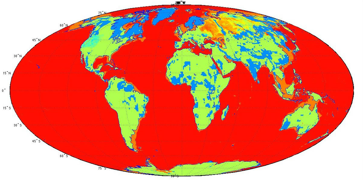
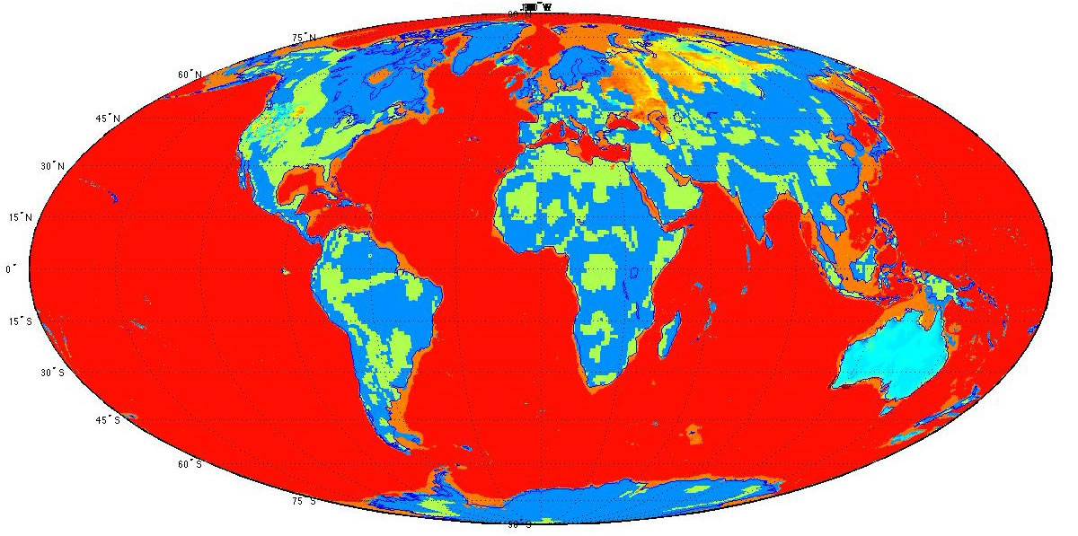
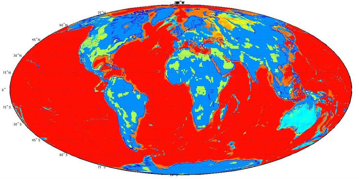
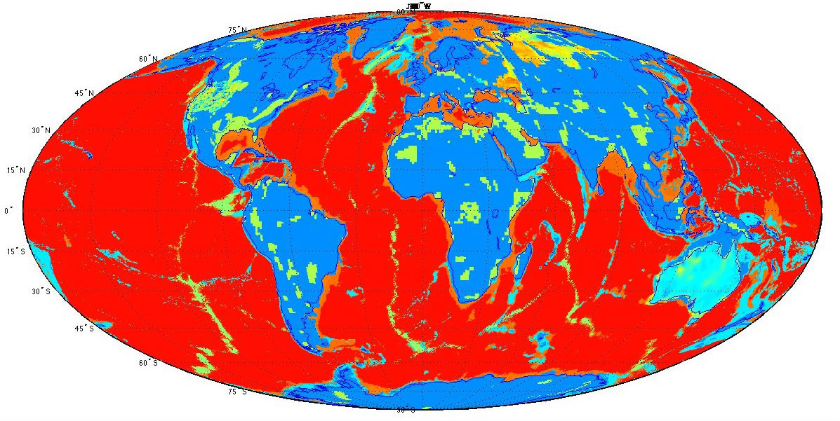
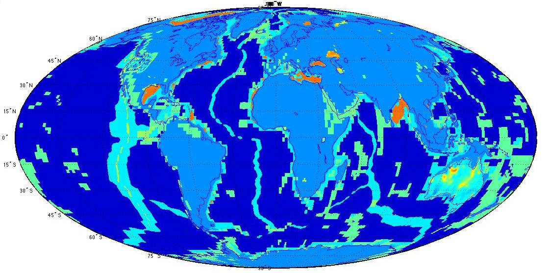
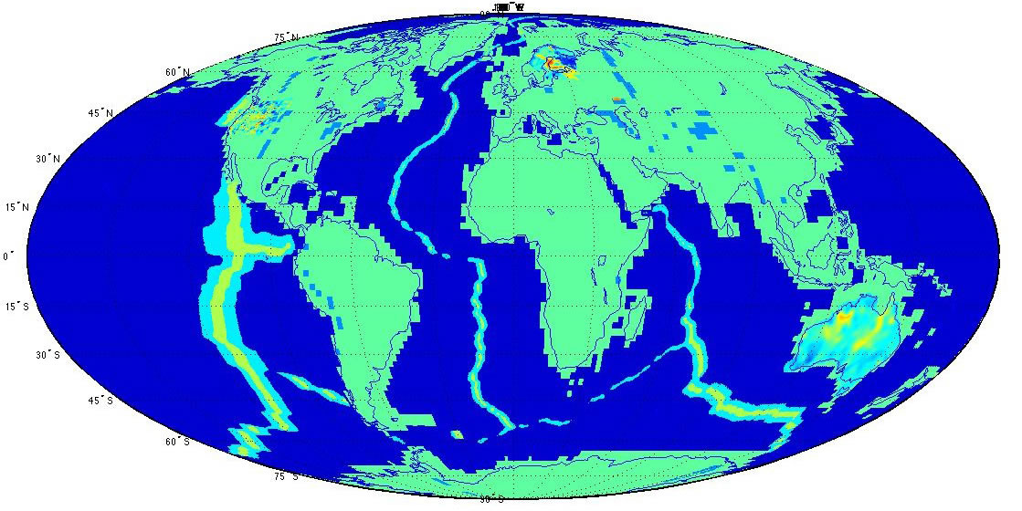
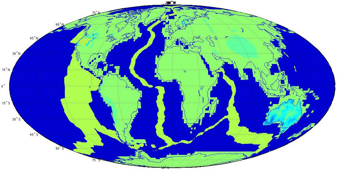
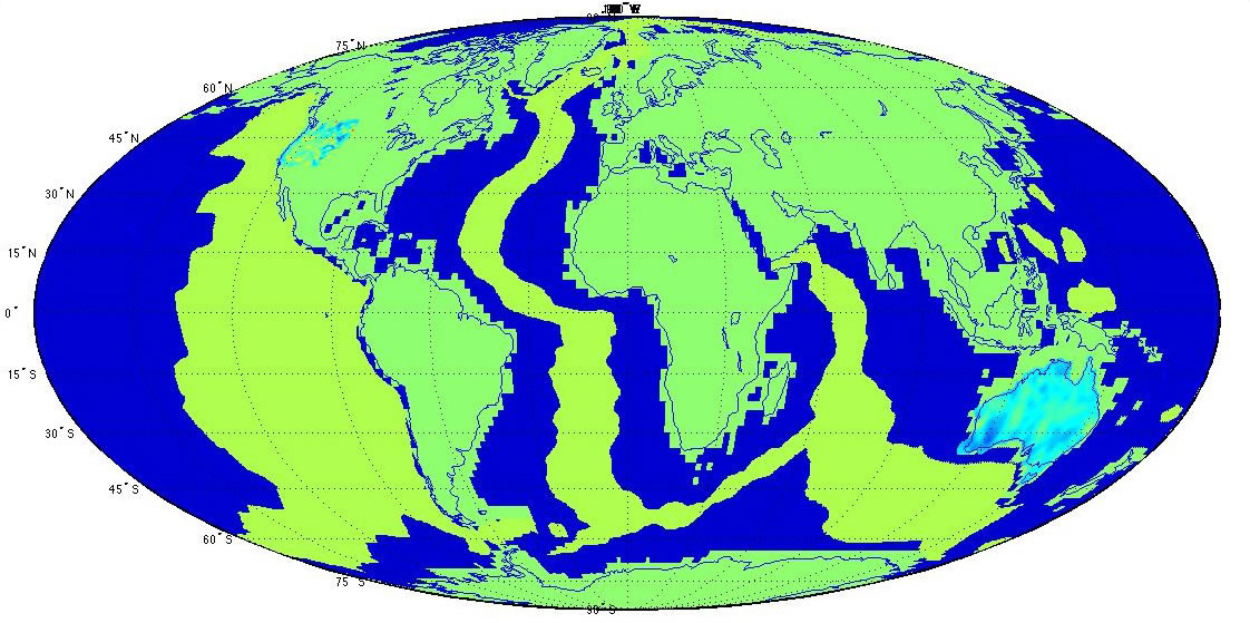
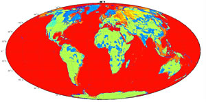
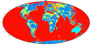
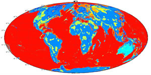
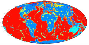
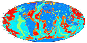
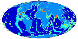
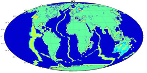
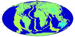
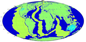
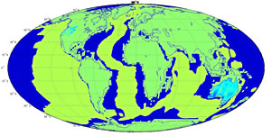
4. GLOBAL CONDUCTIVITY MODEL

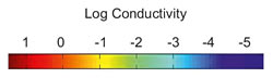	(click image to enlarge)
Depth 0 km	Depth 1 km
Depth 2 km	Depth 3 km
Depth 5 km	Depth 10 km
Depth 20 km	Depth 30 km
Depth 50 km	Depth 75 km
Depth 100 km

5. ACKNOLEDGEMENTS AND REFERENCES

We appreciate the contribution of P. Pushkarev, M.Smirnov, N. Meqbel, T. Lilley, A. Hitchman, T. Korja, N.Narsky and A. Sheinkman for
helpfull discussions and providing conductivity data. The study is funded by Russian Foundation for Basic Research (project 13-05-12111)

REFERENCES:

• Bassin C., Laske G., Masters G., The Current Limits of Resolution for Surface Wave Tomography in North America, EOS Trans AGU 81 (2000)
• Conrad C.P., Lithgow-Bertelloni C. Influence of continental roots and asthenosphere on plate-mantle coupling. Geophys. Res. Let. 33, ( 2006)
• Jones A.G. Imaging the continental upper mantle using electromagnetic methods. Lithos 48, 57–80 (1999)
• Korja T., Engels M., Zhamaletdinov A.A., Kovtun A.A., Palshin N.A., Smirnov M.Yu, Tokarev A.D., Asming V.E., Vanyan L.L., Vardaniants I.L., and the BEAR Working Group. Crustal conductivity in Fennoscandia – a compilation of a database on crustal conductance in the Fennoscandian Shield. Earth Planets Space 54, 535–558 (2002)
• Kuvshinov. A.V. 3-D Global induction in the oceans and solid Earth: Recent progress in modeling magnetic and electric fields from sources of magnetospheric, ionospheric and oceanic origin. Surveys in Geophysics 29,139–186 (2008)
• Kuvshinov. A.V. Deep electromagnetic studies from land, sea, and space: progress status in the past 10 years. Surveys in Geophysics 33,169–209 (2012)
• Meqbel N.M., Egbert G.D., Wannamaker P.E., Kelbert A., Schultz A. Deep electrical resistivity structure of thenorth western U.S. derived from 3-D inversion of US Array magnetotelluric data. Earth and Planetary Science Letters 402,290–304 (2014)
• Puthe C., Kuvshinov A., Towards quantitative assessment of the hazard from space weather. Global 3-D modellings of the electric field induced by a realistic geomagnetic storm. Earth Planets Space 65, 1017–1025 ( 2013)
• Sheinkman A.L., Narsky N.V. Sedimentary cover total conduce map of the territory of Russia. In: Proceedings of the IV All-Russian School-seminar on Electromagnetic Sounding of the Earth, Moscow (2009)
• Vanyan L.L., Shilovsky P.P. Deep electrical conductivity structure of the oceans and continents. Nauka, Moscow (1983)
• Whittaker J., Goncharov A., Williams S., Mulle R.D., Leitchenkov G. Global sediment thickness dataset updated for theAustralian-Antarctic Southern ocean. Geochem. Geophys. Geosys. 14, 3297–3305 (2013)

Phone: +7 (499) 1245996